- 관련 Fluke 회사:
- Fluke
- Fluke Biomedical
- Fluke Networks
- Fluke Process Instruments
Fluke의 더 많은 브랜드 보기
Readout connection
Thermocouple connection to the readout depends whether an internal or external reference junction is used. Internal reference junctions are generally used for high throughput, low-to-medium accuracy applications. There is less opportunity for error and the process is simpler. The limitation in accuracy is due to the additional uncertainty in the reference junction compensation circuit itself (usually an additional 0.05 °C to 0.25 °C).
Internal reference junction connection
Connect the 2-wire thermocouple either directly or through an extension wire to the readout observing polarity. Never use copper for the extension wire, since errors will result. Ensure all connections are tight and clean. Loose and/or dirty connections will cause spurious voltages and measurement errors. Using switches and multiplexors also will result in errors, because these devices are normally constructed of copper. Switches are available that are constructed of thermocouple materials and can be used if a large number of a single type of thermocouple must be calibrated. However, switches constructed of thermocouple materials will still contribute an error that is extremely hard to quantify. If a large quantity of thermocouples must be calibrated, a multi-channel readout or external reference junction technique is recommended.

External reference junction connection
External reference junctions are capable of the highest accuracy and are almost always used for calibration of noble metal (R and S type) thermocouples. They are generally not necessary for the accuracy requirements for base metal thermocouples. External reference junctions must be used when high accuracy is required or the readout is not equipped with internal reference junction compensation (such as a typical DMM). External reference junction connection is slightly more involved with a single unit under test (UUT), but can become quite complicated when several UUTs are being calibrated and uncertainties must be kept to a minimum.
The thermocouple is connected through high-quality copper wires to the readout. The thermocouple-to-copper connections are then immersed into an ice bath to form the reference junction. The connections must be electrically insulated from one another and physically dry. Usually, the wires are welded, soldered, or twisted tightly and protected with heat shrink tubing. The group of wires is inserted into a thin wall metal or glass closed end tube and the tube is inserted into the ice bath. Immersion depth is important and depends upon the wire diameter. Usually, six to twelve inches is sufficient. The copper connecting wires are attached either directly to the readout or through a switch to the readout. Each UUT requires an individual reference junction.
Some UUTs are terminated in thermocouple connectors and cannot be conveniently connected as described. In these cases, “reference junction probes” can be constructed out of copper and thermocouple wire of the type required. The thermocouple end is terminated with connectors which will mate to the UUT connectors. These probes must be calibrated if high accuracy is required. Alternatively, internal reference junction compensation can be used. Frequently, readouts equipped with internal reference junction compensation have thermocouple connectors built in.

All temperature sources have instabilities and gradients. These create calibration errors and/ or uncertainties. Probes should be placed as close together as possible to minimize these effects. In dry-well temperature sources, the probe immersion points are fixed. Baths and open tube furnaces offer flexibility in probe placement. The probes to be calibrated should be placed in a radial pattern with the reference probe in the center of the circle. When using a tube furnace, thermocouples are bundled around a reference thermometer held together with fiberglass core or tape and inserted into the furnace. This placement ensures an equal distance from the reference probe to each of the UUTs.
The sensing elements should also be on the same plane. Thermocouple junctions are usually at the tip of the probe. Sufficient immersion is required so that stem losses do not occur. Generally, immersion is sufficient when the probes are immersed to a depth equal to 15 times the probe diameter plus the length of the sensing element. For example, a 0.25-inch diameter probe with a 1.25-inch long sensing element would need to be immersed a minimum of 5 inches ((15 x 0.25 in) + 1.25 in = 5 in). This rule of thumb is generally correct for probes with thin wall construction and situations with good heat transfer. More immersion is required if the probe has thick wall construction and/or poor heat transfer is present (such as a dry-well with incorrectly sized holes).
Industry standards and guidelines require that a thermocouple be calibrated over the full temperature range in which it is used. Calibration can take substantial time, especially if several thermocouples need to be calibrated. The process involves ramping the temperature source to a setpoint temperature and recording the thermocouple reading when the setpoint temperature is stable. Sufficient time needs to be allowed at each setpoint for the temperature source to achieve stability and uniformity before recording. Then the process is repeated for each setpoint in a series covering the working temperature range of the thermocouple.
The 1586A Super-DAQ includes an “automated sensor calibration” feature that automates the thermocouple calibration process. When the 1586A Super-DAQ is connected to a 9118A Thermocouple Calibration Furnace, the Super- DAQ will control and monitor the 9118A setpoint temperature, read up to 40 thermocouples and automatically collect data when the furnace is stable within parameters defined by the user. The Super-DAQ will then advance the 9118A to the remaining programmed setpoint temperatures, collecting data at each setpoint along the way. Once the test has been configured and started, the technician can walk away to work on other activities. This unique feature, available only from Fluke Calibration, greatly enhances lab productivity and measurement accuracy.
For more information, visit the 1586A Resource Center at www.flukecal.com.
There are two types of thermocouple calibration— characterization and tolerance testing. Most thermocouples are not stable enough for characterization calibration. Typically, thermocouple probes and/or wire are tolerance tested for compliance to American Society for Testing and Materials (ASTM) error ratings. Tolerance testing involves measuring the voltage output at various temperatures and calculating the error from the standard tables.
For most applications, thermocouples are tolerance tested to verify they behave as the standard model predicts within certain limits. The ASTM has two sets of limits called “standard limits of error” and “special limits of error.” The special limits of error use tighter tolerances and were developed to cover the enhanced performance of better grade wire used in more expensive thermocouples. To calibrate a thermocouple to ASTM specifications is to determine that it follows the standard model. Individual thermocouple probes are calibrated in some cases, while entire rolls of wire require certification in other cases. The method is straightforward with no data fitting or complex calculations required.
When tolerance testing will not provide enough information regarding a thermocouple’s voltage response to an applied temperature, a characterization of the thermocouple’s performance throughout its full range provides a more complete analysis. Thermocouple characterization is typically reserved for high accuracy applications involving noble metal thermocouples. Under most circumstances, base metal thermocouples are not stable and will not reproduce the behavior observed during characterization.
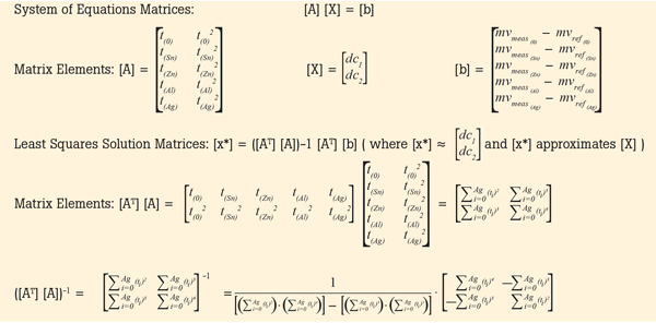
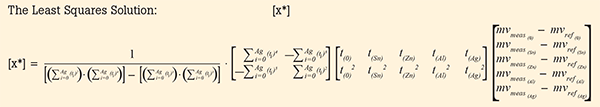
Characterization of a thermocouple involves determining the difference between the measured and standard voltage and then correcting this difference by fitting it to a second order polynomial. Fitting the data is simple in concept but can be complicated in practice. Essentially, the process is to solve a set of simultaneous equations which contain the calibration data to arrive at a set of coefficients unique to the thermocouple and calibration. An accepted “characterization” is based on principles found in NIST Special Publication 250-35, used similarly at Fluke Calibration for the re-certification of Type S and R thermocouples(1).
To formulate the “deviation function,” several linear algebra operations are performed to determine a “least squares solution” to the over-determined system formed by the “FP temperatures and their squared values” and “the voltage differences between the measured values by the thermocouple under test at the FP temperatures” and the corresponding “reference function” voltage values at the same FP temperatures. The least squares solution provides two coefficients which are added algebraically to the corresponding terms in the “reference function” to produce the “thermocouple characterization” function. Refer to Appendix B for a summary of the linear algebra operations.
| Freeze point element or compound | Chemical symbol | ITS-90 freeze point temperature (°C) |
|---|---|---|
| Silver | Ag | 961.78 |
| Aluminum | Al | 660.323 |
| Zinc | Zn | Zinc Zn |
| Tin | Sn | 231.928 |
| Water | H2O | Water H2O |
| (2)NIST Monograph 175, (1993), p.4. | ||
| TYPE B | Pt - 30 % Rh vs. Pt - 6 % Rh | Extension Grade Color = Gray | ||
|---|---|---|---|---|
| Test Temperatures | Type B Sensitivity | Nominal E | Standard Limits Tolerance (± °C) | Special Limits Tolerance (± °C) |
| 1250.00 °C | 10.622 uV/°C | 7.311 mV | 6.25 | 3.13 |
| 1000.00 °C | 9.123 uV/°C | 4.834 mV | 5.00 | 2.50 |
|
Range: 870 °C to 1700 °C; Tolerances:
|
||||
| TYPE E | Ni - Cr vs. Constantan | Extension Grade Color = Purple | ||
|---|---|---|---|---|
| Test Temperatures | Type E Sensitivity | Nominal EMF | Standard Limits Tolerance (± °C) | Special Limits Tolerance (± °C) |
| 870.00 °C | 77.393 uV/°C | 66.473 mV | 4.35 | 3.48 |
| 500.00 °C | 80.930 uV/°C | 37.005 mV | 2.50 | 2.00 |
| 250.00 °C | 76.240 uV/°C | 17.181 mV | 1.70 | 1.00 |
|
Range: -200 °C to 870 °C; Tolerances:
|
||||
| TYPE J | Iron vs. Constantan | Extension Grade Color = Black | ||
|---|---|---|---|---|
| Test Temperatures | Type J Sensitivity | Nominal EMF | Standard Limits Tolerance (± °C) | Special Limits Tolerance (± °C) |
| 760.00 °C | 63.699 uV/°C | 42.281 mV | 5.63 | 3.00 |
| 500.00 °C | 55.987 uV/°C | 27.393 mV | 3.75 | 2.00 |
| 250.00 °C | 55.512 uV/°C | 13.555 mV | 2.20 | 1.10 |
|
Range: 0 to 760 °C; Tolerances:
|
||||
| TYPE K | Ni - 10 % Cr vs. Ni - 5 % (Alumina - Silica) | Extension Grade Color = Yellow | ||
|---|---|---|---|---|
| Test Temperatures | Type K Sensitivity | Nominal EMF | Standard Limits Tolerance (± °C) | Special Limits Tolerance (± °C) |
| 1260.00 °C | 35.566 uV/°C | 51.000 mV | 9.45 | 5.04 |
| 900.00 °C | 40.005 uV/°C | 37.326 mV | 6.75 | 3.60 |
| 600.00 °C | 42.505 uV/°C | 24.905 mV | 4.50 | 2.40 |
| 300.00 °C | 41.446 uV/°C | 12.209 mV | 2.25 | 1.20 |
|
Range: -200 °C to 1260 °C; Tolerances:
|
||||
| TYPE N | Ni - 14 % Cr - 1.5 % Si vs. Ni - 4.5 % Si - 0.1 % Mg | Extension Grade Color = Orange | ||
|---|---|---|---|---|
| Test Temperatures | Type N Sensitivity | Nominal EMF | Standard Limits Tolerance (± °C) | Special Limits Tolerance (± °C) |
| 1260.00 °C | 36.580 uV/°C | 46.060 mV | 9.45 | 5.04 |
| 900.000 °C | 39.040 uV/°C | 32.371 mV | 6.75 | 3.60 |
| 600.000 °C | 38.959 uV/°C | 20.613 mV | 4.50 | 2.40 |
| 300.000 °C | 35.422 uV/°C | 9.341 mV | 2.25 | 1.20 |
|
Range: 0 to 1260 °C; Tolerances:
|
||||
| TYPE R | Pt vs. Pt - 13 %Rh | Extension Grade Color = Green | ||
|---|---|---|---|---|
| Test Temperatures | Type R Sensitivity | Nominal EMF | Standard Limits Tolerance (± °C) | Special Limits Tolerance (± °C) |
| 1084.62 °C | 13.575 uV/°C | 11.640 mV | 2.71 | 1.09 |
| 961.78 °C | 13.065 uV/°C | 10.003 mV | 2.40 | 0.96 |
| 660.32 °C | 11.641 uV/°C | 6.277 mV | 1.65 | 0.66 |
| 419.53 °C | 10.480 uV/°C | 3.611 mV | 1.50 | 0.60 |
| 231.93 °C | 9.168 uV/°C | 1.756 mV | 1.50 | 0.60 |
|
Range: 0 to 1480 °C; Tolerances:
|
||||
| TYPE S | Pt vs. Pt - 10 %Rh | Extension Grade Color = Green | ||
|---|---|---|---|---|
| Test Temperatures | Type S Sensitivity | Nominal EMF | Standard Limits Tolerance (± °C) | Special Limits Tolerance (± °C) |
| 1084.62 °C | 11.798 uV/°C | 10.575 mV | 2.71 | 1.09 |
| 961.78 °C | 11.418 uV/°C | 9.148 mV | 2.40 | 0.96 |
| 660.32 °C | 10.398 uV/°C | 5.860 mV | 1.65 | 0.66 |
| 419.53 °C | 9.638 uV/°C | 3.447 mV | 1.50 | 0.60 |
| 231.93 °C | 8.711 uV/°C | 1.715 mV | 1.50 | 0.60 |
|
Range: 0 to 1480 °C; Tolerances:
|
||||
| TYPE T | Cu vs. Constantan | Extension Grade Color = Blue | ||
|---|---|---|---|---|
| Test Temperatures | Type T Sensitivity | Nominal EMF | Standard Limits Tolerance (± °C) | Special Limits Tolerance (± °C) |
| 370.00 °C | 60.928 uV/°C | 19.030 mV | 2.78 | 1.48 |
| 200.00 °C | 53.150 uV/°C | 9.288 mV | 1.50 | 0.80 |
| 100.00 °C | 46.785 uV/°C | 4.279 mV | 1.00 | 0.50 |
|
Range: -200 °C to 370 °C; Tolerances:
|
||||
Using Transpose and Inverse Identity Matrices, a least squares solution “x*” for the equation in step 4 has the following form: [x*] = (([AT] [A])-1) [AT] [b] (5).
The matrix equations in steps 4 and 5 were adapted from the information in reference (5), pp. 50-54.
EMFref = c0 + (c1)·t90 + (c2)·t90 2 + (c3)·t90 3 +…+ (c8)·t90 8 (where EMF is in μVdc, and t90 is in °C).
EMFdev = 0 + (dc1)·t90 + (dc2)·t902
EMFchar = c0 + (dc1 + c1)·t90 + (dc2 + c2)·t902 + (c3)·t903 +…+ (c8)·t90 (6)
How to Select Thermocouple Calibration Equipment
Calculating Uncertainties in a Thermocouple Calibration System
Thermocouple calibrator selection guide
5649 / 5650 Type R and Type S Thermocouple Standards
Customer and technical support